Working with databases: connect, query, and import

25 minutes · For anyone who pulls data from a SQL database and wants to analyze it without exporting to CSV first. Tutorial 2 helps but isn’t required.

Most workflows that involve a database also involve a second tool. You browse and query in a database client — dBeaver, DataGrip, pgAdmin — then export a CSV, switch to a spreadsheet or a notebook, and start the analysis over there. MathJet collapses that split. It has a database client built into the workspace: connect to SQLite, PostgreSQL, MySQL/MariaDB, SQL Server, or Oracle, browse the schema as a tree, open tables in editable worksheets, and run SQL with results shown as tables — and then everything you’ve learned in the other tutorials applies directly, because a query result or a table is just more data in the same fused workspace. Pull any table or query result into the shared data frame as a variable using the same Create Variable dialog you used for cell ranges in Tutorial 2, chart it, script over it in Python or Jet.

One idea runs through the whole tutorial: edits are deferred. When you change a value in a database table, MathJet updates a local cache — and any charts or variables linked to it — but it does not touch the database. Your edits are committed only when you explicitly Save. That means you can explore, edit, and experiment freely, and nothing reaches the live database until you decide it should.

What you’ll learn

• How to open a database connection from the Data Source Pane — the SQLite path (just a file) and the server path (host, port, credentials)
• How to browse a connection’s tables and columns as a tree
• How to open a table in a specialized worksheet, edit rows and cells, and how the cache-versus-commit model keeps your edits out of the database until you Save
• How to inspect and edit a table’s column schema (types, nullability, primary keys) in the column-list view
• How to run SQL in the SQL script pane and read the results as tables
• How to import a table or query result as a variable with the Create Variable dialog, and chart it
• How to Save pending edits back to the database, and Save the whole database out to a new file

What you’ll need

• MathJet installed (download)
• (Recommended) Tutorial 2 — you’ll reuse the Create Variable dialog and the shared data frame from it
• The sample database: chinook.db — the classic Chinook digital-music-store schema (artists, albums, tracks, invoices, customers). SQLite, no server required.
• (Optional) a PostgreSQL / MySQL / SQL Server / Oracle database of your own, plus its connection details, if you want to try a server connection

---

Step 1: Connect to a database

Download chinook.db and save it somewhere you’ll find it.

Find the Data Source Pane in the top-left of the MathJet window (tabbed with the Workspace Manager and the File Browser). On its toolbar, click the Import Data button — the first button on the toolbar — and choose From Database from the drop-down menu. A dialog titled Connect to a Database opens.

Because SQLite is a single file with no server, its connection is the simplest one:

1. Set Database Type to SQLite.
2. For Database File, browse to the chinook.db you just downloaded.
3. Click Connect (or OK).

A new connection node appears in the Data Source Pane, named for the database.

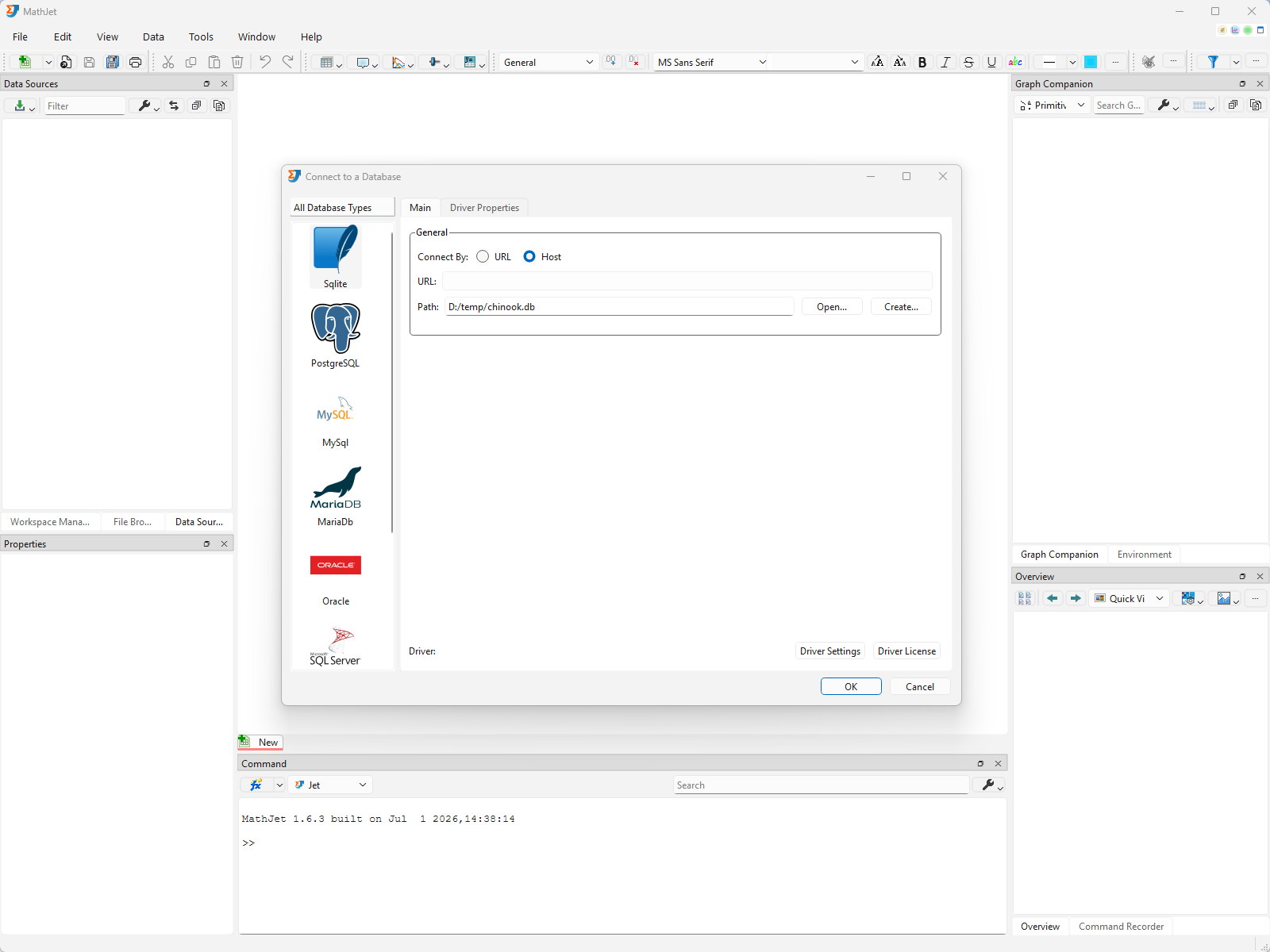
Connecting to a server database instead. For PostgreSQL, MySQL/MariaDB, SQL Server, or Oracle, pick the matching Database Type and the dialog swaps the single file field for the server fields: Host, Port, Database Name, and a Username / Password pair (with an option to save the password). Fill those in and connect. Everything after this step — browsing, editing, querying, importing — works identically regardless of which engine you connected to; only this first dialog differs.

Step 2: Browse the tables and columns

Expand the new connection node in the Data Source Pane. Underneath it, MathJet lists the database’s tables as child nodes — albums, artists, customers, genres, invoices, invoice_items, tracks, and the rest of the Chinook schema.

Expand a table node — say invoices — and its columns appear as their own nodes: InvoiceId, CustomerId, InvoiceDate, BillingCountry, Total, and so on. This is the same tree-of-schema view you’d get from a standalone database client, living right inside the MathJet workspace.

Clicking a node doesn’t just navigate — it previews. Exactly like the Workspace Manager in Tutorial 1, the Data Source Pane drives the Overview Pane and the Properties Pane as you click:

• Click the invoices table node — the Overview Pane renders a colorful heatmap of the table’s values, and the Properties Pane shows summary statistics for the whole table.
• Click a numeric or date column like CustomerId or InvoiceDate — the Overview Pane switches to a line plot of that column’s values.
• Click a categorical column like BillingCountry — the Overview Pane switches to a count histogram of the category values.

The Properties Pane’s statistics update on every click, so you can size up a table or a column before ever opening it.

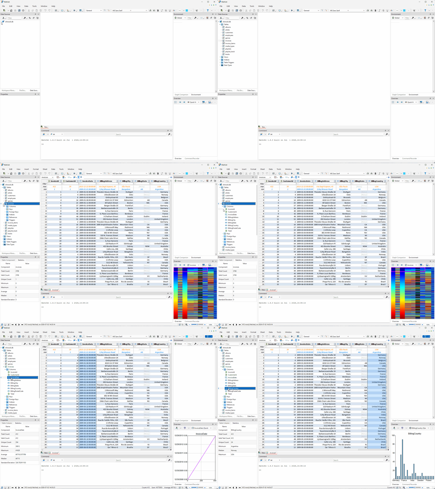
The tree is a navigator, not a data dump — MathJet doesn’t pull a table’s full row set until you actually open it. That keeps the pane responsive even on databases with large tables.

Step 3: Open a table and edit it

Double-click the genres table node (it’s small — 25 rows — which makes it easy to see what’s happening). The table opens in a specialized worksheet: a grid of the table’s rows and columns, with a status bar at the bottom summarizing the table.

Now edit a value. Click the Name cell for the Rock genre and change it to Rock & Roll. Press Enter.

Here’s the key behavior. The cell updates, the status bar notes that the table has unsaved changes, and any chart or variable linked to this table updates too — but the database itself is untouched. Your edit lives in MathJet’s local cache of the table. This is true for every kind of table edit:

• Edit a cell — the new value goes into the cache.
• Insert a row — right-click a row and choose Insert Row; a blank row is added to the cache.
• Delete a row — the row is marked for deletion in the cache.

None of it reaches the database until you Save (Step 8). Until then you can keep experimenting, and you can always discard the pending edits by reloading the table.

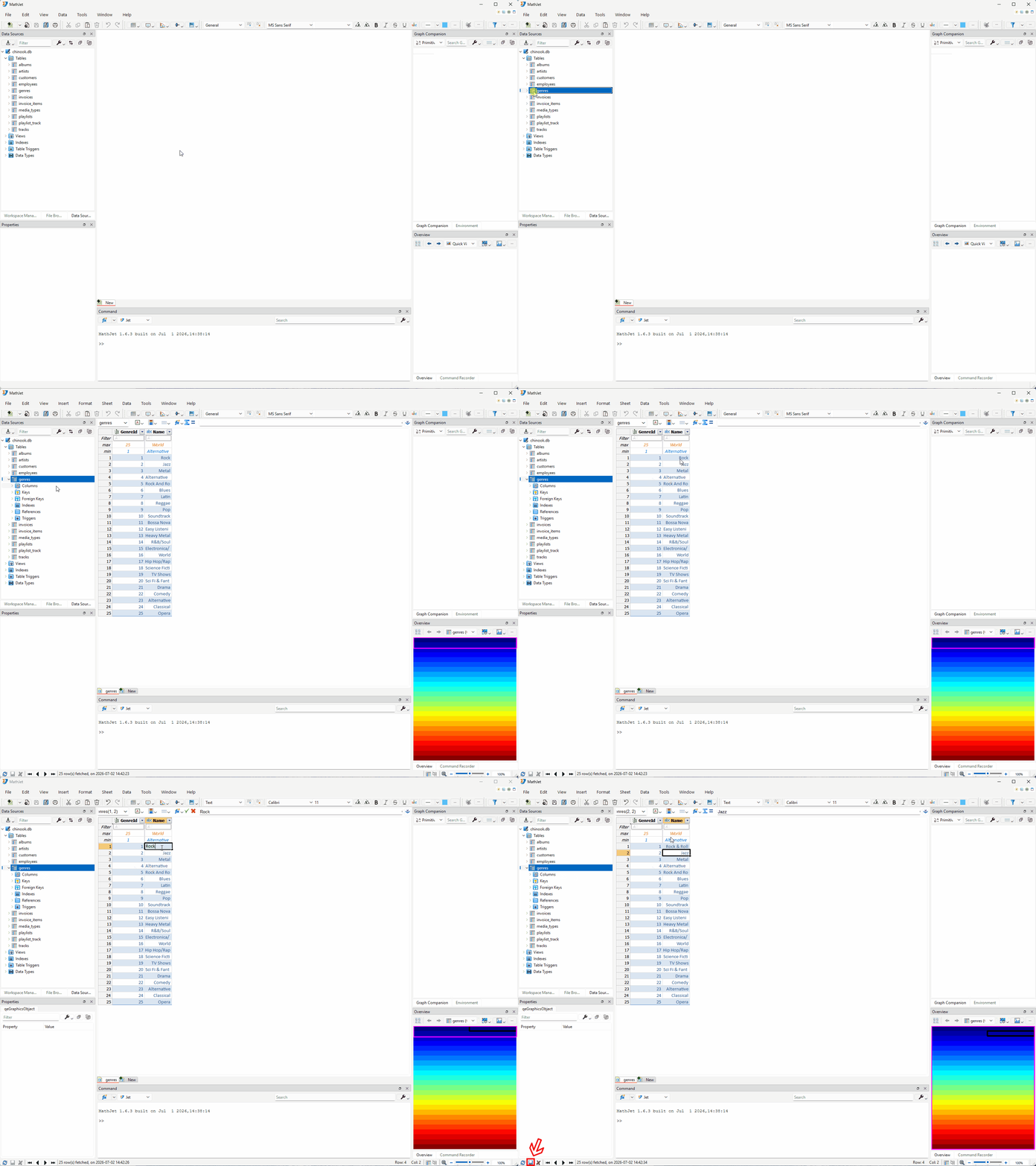
Why deferred edits? A database is shared, durable state — an accidental keystroke shouldn’t rewrite it. MathJet treats the table worksheet like a working copy: edit freely, see the consequences ripple through linked charts and variables, and commit deliberately. It’s the same reason a good editor doesn’t write every keystroke straight to disk.

Step 4: Inspect and edit the column schema

The same table worksheet can show you the table’s structure instead of its rows. Switch to the column-list view (the schema toggle on the sheet’s toolbar). Now each row of the sheet describes one column of the table:

• Name — the column name.
• Type — the declared SQL type (INTEGER, NVARCHAR(120), …).
• Nullable — whether the column allows NULL.
• Primary Key — whether it’s part of the primary key.
• Default — the column’s default expression, if any.

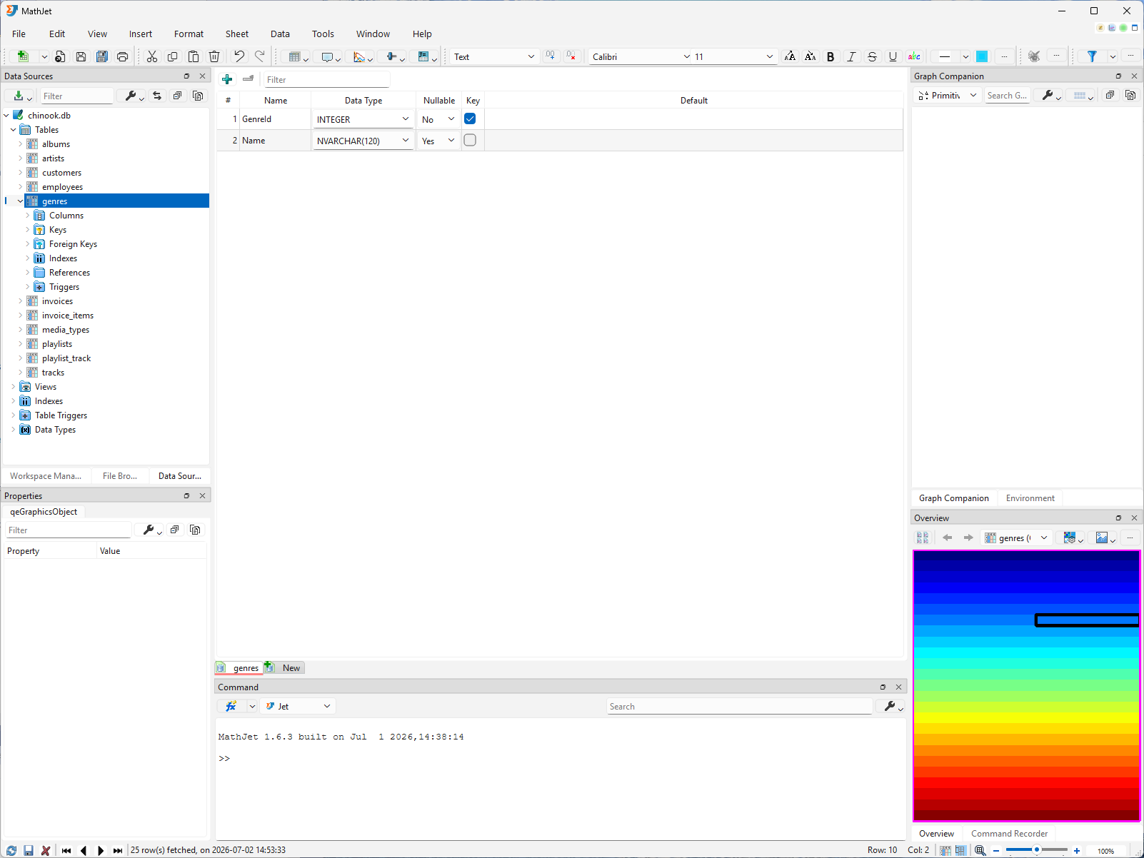
Structural edits work here the same deferred way as data edits. You can rename a column, add a new one (name, type, nullability, default), or drop one, and the changes are held as pending ALTER TABLE operations — applied to the database only on Save, after the row edits, in the same transaction. For now just look; leave the schema unchanged.

Switch back to the row view when you’re done.

Step 5: Run a SQL query

Browsing and editing cover a lot, but the real power of a database is SQL. Open a SQL script pane for the connection (right-click the connection node and choose New SQL Script, or use the SQL Script toolbar button). The pane splits into two: a SQL editor on top and a results area on the bottom.

Type a query that aggregates across a few tables — total revenue per genre:

SELECT g.Name AS Genre,
       SUM(ii.UnitPrice * ii.Quantity) AS Revenue
FROM invoice_items ii
JOIN tracks t ON t.TrackId = ii.TrackId
JOIN genres g ON g.GenreId = t.GenreId
GROUP BY g.Name
ORDER BY Revenue DESC;

Run it — click Execute (or press the run shortcut). The bottom of the pane fills with a result table: one row per genre, a Genre column and a Revenue column, sorted high to low. A status line reports how many rows came back. (To run just one statement out of several, select it first and use Execute Selection — only the highlighted SQL runs.)

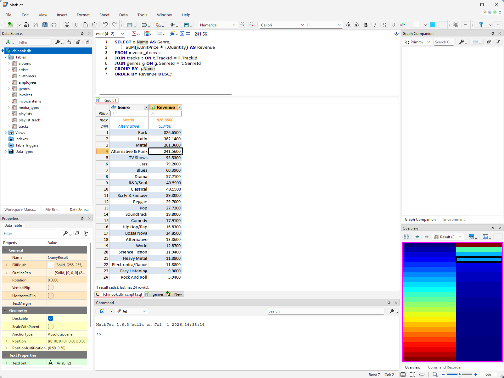
The query runs against the database, not against your cached table edits. So the Rock → Rock & Roll rename you made in Step 3 does not appear in this result — the genre still reads Rock here, because that edit hasn’t been Saved yet. You’ll see it change after Step 8. This is the cache-versus-commit split made concrete: worksheet edits live in the cache; SQL sees the committed database.

Step 6: Chart a result and import it as a variable

A query result is just data in the workspace, so you can visualize it and pull it into the shared data frame like anything else.

Chart it. Select the Genre and Revenue columns in the result table, then insert a chart: Insert → Chart → Column Graph → 2D Column (or the Insert Chart tool button). A column chart of revenue by genre appears — vertical columns with Rock towering over the rest, the long tail falling away to the right. (In MathJet, as in Excel, a column graph has vertical bars; a bar graph has horizontal ones.)

Import it as a variable. To capture the entire result table, click the corner label at the top-left of the result grid — the box above the first row number and left of the first column header — to select the whole table. Then choose Data → Create Variable, the same dialog you used in Tutorial 2 for cell ranges. The Data Source field is pre-filled from the query result instead of a worksheet range; name the variable genre_rev and click OK. It appears in the Environment Pane as a Data Frame — a two-column table of genres and their revenue — ready for scripting.

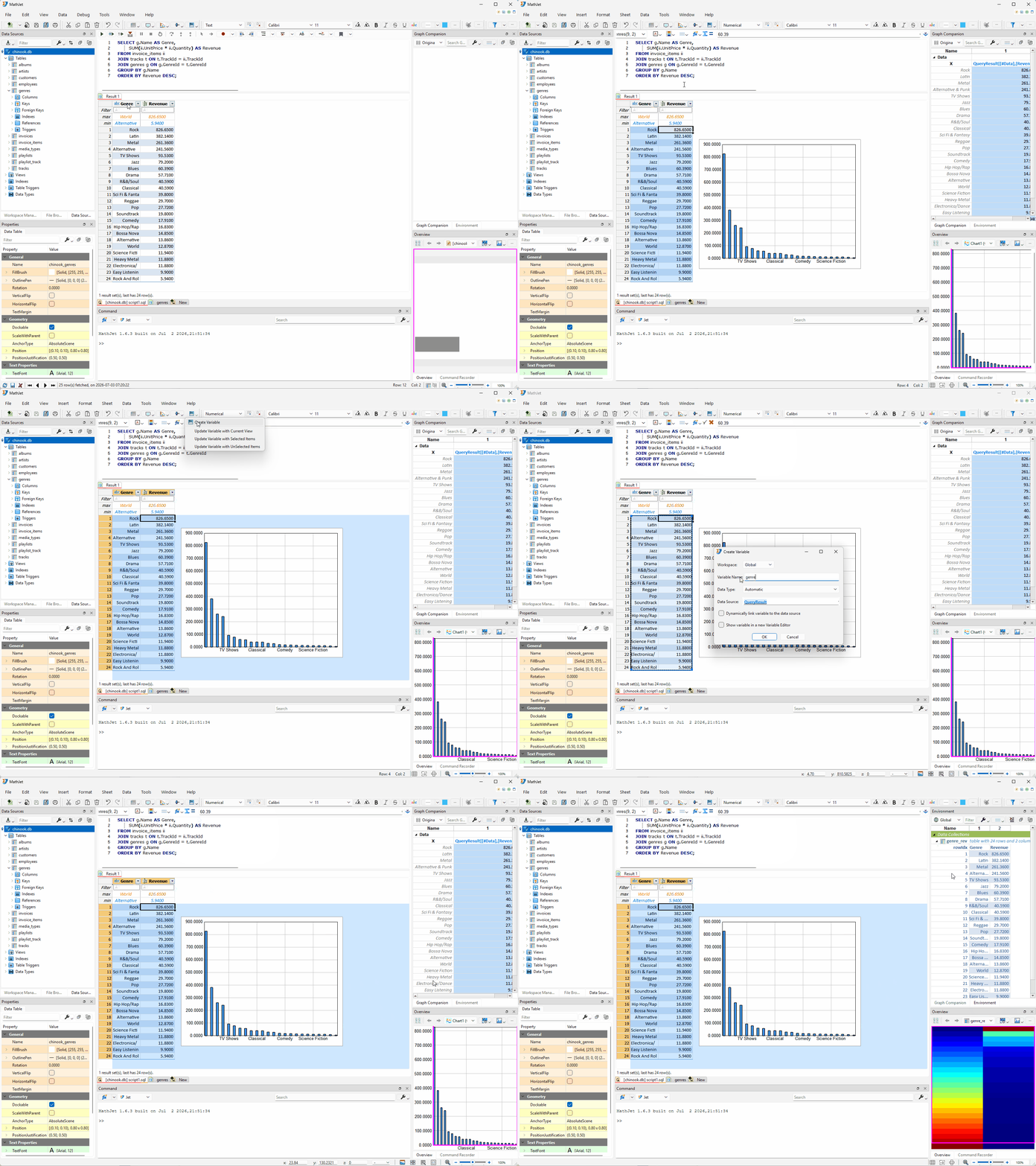
A query result is a snapshot taken when the query ran — it isn’t a live link back to the database (the aggregation doesn’t correspond to any single stored row). That’s the right behavior for a derived, aggregated result: genre_rev is yours to analyze without any risk of writing back. (When you want a live variable that tracks a table, create it from a table worksheet instead — that links to the cache, which commits on Save.)

Step 7: Analyze the imported data

Now genre_rev is an ordinary variable in the shared data frame, reachable from any interpreter. Open the Command Editor and switch it to Python (see Tutorial 2 if you need a refresher on switching languages).

Because it’s a Data Frame, genre_rev arrives in Python as a pandas DataFrame with Genre and Revenue columns. A few things to try:

# Total revenue across all genres
genre_rev["Revenue"].sum()

# The top five genres by revenue
genre_rev.sort_values("Revenue", ascending=False).head(5)

The point isn’t the specific functions — it’s that data you pulled from a SQL query two steps ago is now a first-class Python object, no CSV export in between. Everything you learned in Tutorials 2 through 7 applies to it: mix it with worksheet data, run R on it, feed it into a curve fit, build a dependent graph from it.

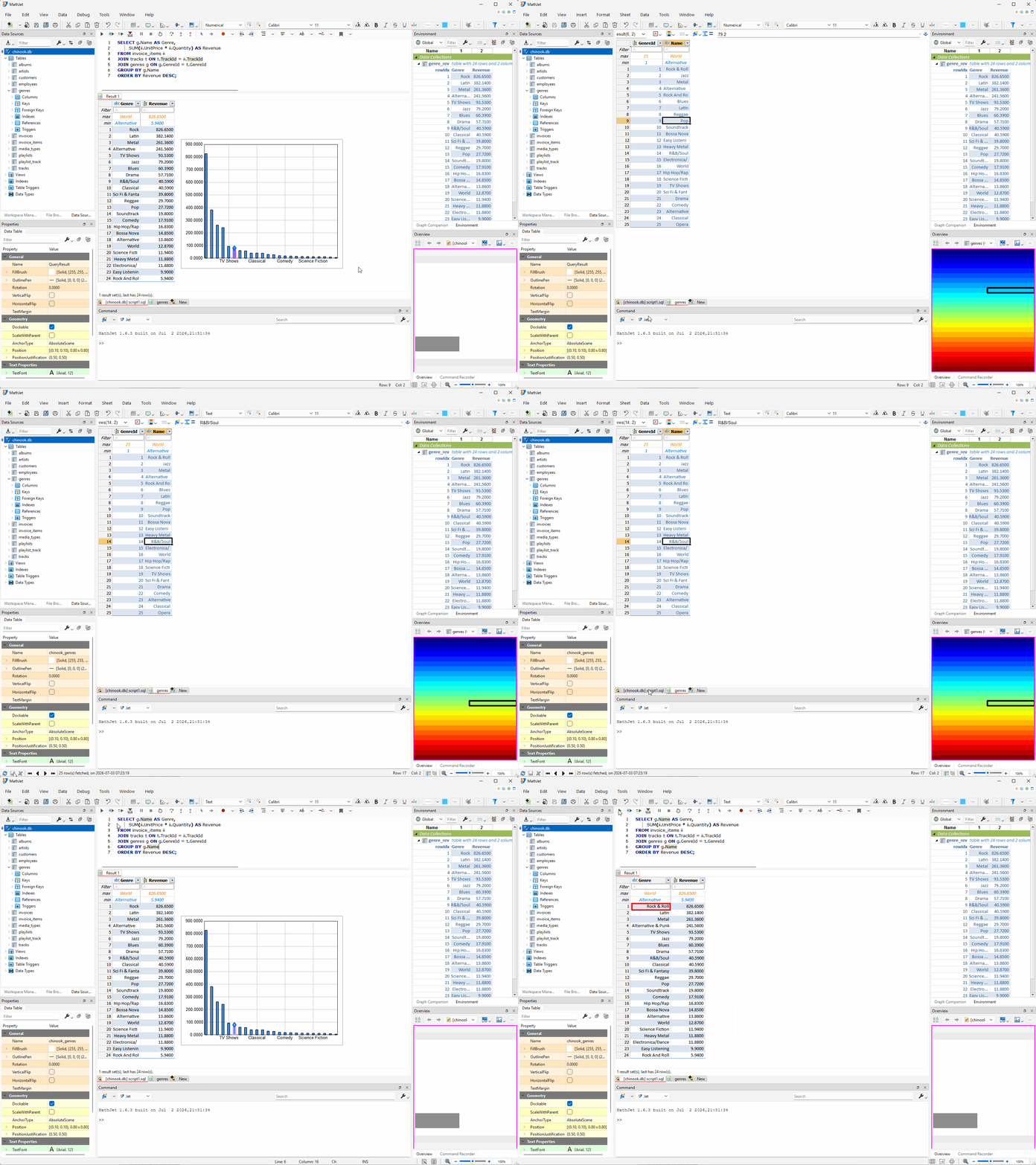
Step 8: Save your changes back to the database

Time to commit the edit from Step 3. With the genres table worksheet active, click the Save Changes button in the status bar — the same status bar that’s been flagging “unsaved changes.” MathJet flushes that table’s pending change set to the database in a single transaction, and your Rock → Rock & Roll rename becomes an UPDATE against the real table. The marker clears.

The Save Changes button commits only the currently active database table. To commit pending edits across all open database tables in one go, use File → Save (or Ctrl+S) instead — it saves the whole workspace, database tables included.

Confirm it committed: go back to the SQL script pane and re-run the revenue-by-genre query from Step 5. This time the top row reads Rock & Roll — the query now sees your edit, because it’s part of the database. That round trip, edit → Save → query reflects it, is the whole cache-versus-commit model in one motion.

Saving the database to a new file. For a file-backed database like SQLite, File → Save As writes the entire database out to a new .db file — a clean copy, useful for snapshots or handing off a modified database. (Server databases — PostgreSQL, SQL Server, and the rest — have no single file to copy, so Save As to a file isn’t offered for them; their changes are committed in place on Save.)

What you’ve learned

• Connecting — the Data Source Pane opens connections to SQLite, PostgreSQL, MySQL/MariaDB, SQL Server, and Oracle. SQLite needs only a file; server engines take host, port, database name, and credentials. Everything downstream is engine-independent.
• Browsing — a connection expands into a tree of tables, and each table into its columns, without loading any rows until you open a table.
• Editing with deferred commit — cell edits, row inserts, and row deletes accumulate in a local cache and propagate to linked charts and variables, but reach the database only when you Save.
• Schema view — the column-list view shows and edits table structure (rename / add / drop columns), applied as ALTER TABLE operations on Save.
• Querying — the SQL script pane runs arbitrary SQL (all of it, or just the selection) against the connection and shows results as tables. Queries see the committed database, not your unsaved cache edits.
• Importing — a query result or a table becomes a workspace variable through the same Create Variable dialog used for cell ranges; from there it’s a first-class object for charting and polyglot scripting.
• Saving — the Save Changes button in the status bar commits the active table’s pending edits transactionally; File → Save commits every open database table at once; Save As writes a file-backed database out to a new file.

Next steps

Databases are one of several ways to get external data into MathJet. For spreadsheet files, see Reading and writing real Excel files — the sibling “external data in” tutorial. To go deeper on the variables you imported here — mixing them across Jet, Python, and R — revisit Mixing languages in formula bar and scripts.

Once your query results are in the workspace, the visualization and analytics tutorials apply directly: Interactive plots for axis folding and data grouping, and Graph analytics for characteristics tables, curve fits, and dependent graphs.

For the reference on connections, table sheets, and the SQL script pane, see the Data Source Window reference.

Troubleshooting

I don’t see the Data Source Pane. By default it sits in the top-left of the MathJet window, tabbed with the Workspace Manager and the File Browser — click its tab to bring it forward. If it’s been closed entirely, reopen it from Window → Tool Windows → Data Source Pane.

The Connect to a Database dialog can’t open my SQLite file. Make sure the path points at the .db file itself and that the file isn’t open with an exclusive lock in another program. A database opened read-only (e.g., on read-only media) can be browsed and queried but not saved.

A server connection fails. Double-check host, port, database name, and credentials, and confirm the server accepts connections from your machine (firewall, and the server’s own host-based access rules). The connection dialog reports the driver’s error message — read it; “authentication failed” and “could not connect to host” point at very different fixes.

My table edits don’t show up when I query the table. That’s expected. SQL runs against the database; your unsaved edits live in the cache. Save the table first — the Save Changes button in the status bar, or File → Save — then re-run the query. Until you save, the query reflects the committed state.

Save reports it can’t identify a row to update. To turn a cached edit into an UPDATE or DELETE, MathJet needs to identify the original database row — by its primary key, or by an implicit row id (SQLite rowid, PostgreSQL ctid) when the table has no primary key. A view or a table with neither can be read but not edited in place; query the underlying base tables instead.

Create Variable is grayed out on a query result. Select the result columns (or cells) first — the command acts on a selection, the same as it does for worksheet cell ranges in Tutorial 2.