R / RStudio: bringing your R workflows into MathJet®

25 minutes · For users coming from R or RStudio. Working R experience required.

This tutorial mirrors the structure of Tutorial 3: MATLAB scripts and Tutorial 4: Jupyter notebooks, substituting R for the host language. If you’ve completed either of those, the workflow here will feel familiar.

R has a deep statistical-modeling stack — survival analysis, mixed-effects models, the formula-language lm()/glm() family, the entire CRAN ecosystem. Python doesn’t fully duplicate any of this. If R is where you do your statistical work, the question is whether MathJet can host it without making you give anything up. This tutorial answers that on a real R workflow: open an R script in MathJet, run it in MathJet’s embedded R interpreter (same memory as Python and Jet — no rpy2, no reticulate, no inter-process serialization), inspect variables the way you would in RStudio’s Environment Pane, watch a ggplot2 plot become an interactive MathJet chart, edit data in the Variable Editor with changes flowing back to the interpreter, and extend the workflow with a Python step that sees the same variables — without leaving the session.

Before you start

1. MathJet installed. Download for your platform.
2. R installed with required packages. MathJet does not ship R — it expects a working R installation on your system. You’ll need base R plus the dplyr and ggplot2 packages. Install them from R if you haven’t already: install.packages(c("dplyr", "ggplot2")).
3. The sample script and data. Download statistical_analysis.R and the companion measurements.csv. Put them in the same folder. The script is about forty lines: it loads measurements.csv with read.csv(), computes per-condition summary statistics with dplyr, runs a one-way ANOVA with aov() and Tukey HSD post-hoc comparisons, computes Cohen’s d, and draws a ggplot2 boxplot with jittered points.
4. R basics. You should be comfortable with data.frames, dplyr, and basic ggplot2. The tutorial doesn’t introduce R from scratch, but doesn’t assume advanced R knowledge either.
5. R version. MathJet supports R 4.0 and later. Older R versions may work but aren’t regularly tested.
6. (Optional) RStudio. Useful if you want to run the same script in both environments and compare behavior side-by-side. Not required to complete the tutorial.

Step 1: Look at the script

Open statistical_analysis.R in any text editor (or in MathJet — we’re about to). The script does four things:

1. Loads measurements.csv with read.csv() and prints the row/column counts.
2. Summarizes the data by condition group using dplyr::summarise() — count, mean, standard deviation, standard error.
3. Runs an ANOVA with aov(measurement_value ~ condition, data = df), followed by TukeyHSD() for pairwise comparisons and a manual Cohen’s d calculation for treatment_a vs control.
4. Draws a ggplot2 boxplot with jittered points, colored by condition — geom_boxplot() + geom_jitter(), with theme_minimal().

Step 2: Run the script in MathJet

Launch MathJet, then either:

• Drag statistical_analysis.R from your file manager into MathJet’s main window, or
• Use File → Open and pick the script.

MathJet opens the file in a script editor view with R syntax highlighting. There’s no “select language” dialog — .R files are recognized by extension and routed to MathJet’s embedded R interpreter automatically. MathJet detects your system’s R installation and runs the interpreter embedded in its own process — same memory space as the Python and Jet interpreters, no inter-process serialization.

Click Run (or press F5). MathJet sources the entire script. You’ll see:

• Text output in the Command Editor at the bottom — the summary statistics table, the ANOVA table, the Tukey HSD pairwise comparisons, and the Cohen’s d value.
• The Environment Pane on the right populates with the script’s variables: df, summary_stats, model, tukey, control, treatment_a, pooled_sd, cohens_d.

Notice that the ggplot2 boxplot does not appear yet. This is standard ggplot2 behavior — when a ggplot call runs inside a sourced script, ggplot2 builds the plot object but does not render it. The same thing happens in RStudio. To see the chart, select the ggplot function call at the end of the script (the ggplot(df, ...) block, lines 40–46) and press Run again (or use Run → Run Selection). Now a chart sheet appears with the boxplot — and it’s not a static image. More on that in Step 5.

Step 3: Verify the output against RStudio (optional)

If you ran the script in RStudio earlier, compare:

• The ANOVA p-value, the Tukey HSD pairwise comparisons, and the Cohen’s d value printed in MathJet’s Command Editor should match RStudio’s console output to within numerical-precision noise (typically identical to ~12 decimal places).
• The ggplot2 boxplot’s data distribution should be identical; default colors and fonts will differ because MathJet renders ggplot2 output through its own plotting engine, but the data being plotted is the same.

If anything differs in a way you can’t explain by floating-point precision, that’s a real compatibility issue worth reporting — see Troubleshooting at the bottom.

Step 4: Inspect the workspace variables

If you’ve used RStudio, the Environment Pane should feel familiar — it’s the same idea: a live list of every object in the R workspace, updated after each execution. But MathJet’s version is richer because it feeds the Overview Pane and integrates with the Variable Editor and spreadsheet.

Click around. Click cohens_d in the Environment Pane. The Overview Pane (lower-right) displays the single scalar value. Click control (a numeric vector of 25 measurements) — the Overview Pane shows a line plot. Click df — the Overview Pane renders a heatmap preview of the data.frame, each column on its own auto-computed color scale. The Overview Pane picks a shape-appropriate view for whatever you click.

Explore the columns. Click the expansion button on the left of the df header name to expand the variable cell block. Now click the condition column header. The Overview Pane switches to a histogram showing the count for each condition group. Click measurement_value — a distribution plot. Double-click the condition histogram in the Overview Pane to promote it to a new figure tab in the main window’s central tab area.

Inspect statistical model objects. Click model (the aov output) in the Environment Pane. The Overview Pane shows basic structure information — the object is a list, with a count of its child elements. Click the expansion button to expand model into a tree. Each child element (residuals, coefficients, effects, etc.) appears as a node; compound children like vectors, matrices, or nested lists can be expanded further — there’s no limit to the depth. Click tukey and expand it the same way to see the TukeyHSD pairwise comparison structure. This tree-based inspection works for any R list or nested object, though it’s most useful for well-structured outputs like model results.

This is the same adaptive visualization you’d see in Tutorial 1 and Tutorial 3 — the Environment Pane and Overview Pane work identically regardless of which language created the variable.

Step 5: ggplot2 becomes an interactive MathJet chart

Switch to the chart sheet that appeared when the script ran. The ggplot2 boxplot is not a static image — MathJet intercepted the ggplot2 output and rendered it as a native MathJet chart, the same kind of interactive chart you’d create from the GUI.

Zoom. Click the chart first to give it focus, then scroll the mouse wheel — the chart zooms in, centered on the cursor. Scroll backward to zoom out. Shift-drag to pan.

Graph Companion. The Graph Companion table (tabbed behind the Environment Pane) shows a specialized boxplot table with the key statistical values for each condition group: Low Whisker, Quantile 1, Median, Quantile 3, High Whisker. Click any data cell in this table — the corresponding symbol appears on the boxplot, highlighting the exact value on the chart.

The R code that created the plot didn’t change. The ggplot() + geom_boxplot() + geom_jitter() calls are identical to what you’d write in RStudio. MathJet’s R interpreter intercepts the ggplot2 output at render time and presents it as a native chart instead of rasterizing to a static image. The interactivity is a property of the runtime, not of the script.

You’re in control of the conversion. A few related controls:

• The Options tool button (last on the notebook toolbar) toggles whether ggplot2 figures auto-convert to MathJet charts.
• Click inside a figure to give it focus; a row of buttons appears at the top-right corner.
• From those buttons: toggle between the static image and the interactive chart, maximize/restore, or replicate the chart as a separate figure tab or floating window.

Step 6: Open in the Variable Editor, write formulas

Double-click the df header name in the Environment Pane. MathJet opens df in a Variable Editor tab — a specialized spreadsheet that shows the data.frame’s column names, row indices, and all data values. This is a live, editable view: changes here write back to the R interpreter’s df immediately.

Write a formula. Click a cell outside the data area. Select all data rows in the measurement_value column — MathJet shows the reference as df[#DATA, [measurement_value]] in the formula bar, using Excel table reference format. Type a formula like =AVERAGE(df[#DATA, [measurement_value]]) in the cell. You now have an R-produced data.frame visible in a spreadsheet alongside Excel formulas.

Create a chart. Select the columns you want to plot, then use Insert → Chart. The chart is a full MathJet interactive chart. If you re-run the script and df changes, the Variable Editor updates and any chart sourced from those columns redraws.

Step 7: Edit and filter data, see it in the script

The link between the Variable Editor and the R interpreter runs both directions.

Edit a value. In the Variable Editor, pick a cell in the measurement_value column — say, row 10 — and type a different value (e.g., 999). Press Enter. Switch to the Command Editor at the bottom, make sure R is selected, and type:

summary(df$measurement_value)

The output reflects the change — the mean shifted because one value is now 999. The edit flowed from the Variable Editor through the shared variable store to R. Switch to the chart sheet with the ggplot2 boxplot — the chart has redrawn too. The boxplot’s distribution shift is subtle for a single-value change, but the jittered scatter points are more noticeable: all points shift position because geom_jitter() reapplies random offsets on each redraw.

Undo to restore. Press Ctrl+Z in the Variable Editor to undo the value edit, restoring df to its original state.

Filter with Apply to original data. Click the dropdown button on the right side of the condition column header. A filter menu opens showing a list of all unique values (control, treatment_a, treatment_b, treatment_c) with checkboxes. At the bottom of the menu, check “Apply results to original data”. Uncheck treatment_c and click OK.

Because “Apply results to original data” is checked, MathJet removes all rows where condition == "treatment_c" from the actual df data.frame. Run nrow(df) in the Command Editor — it shows 75 instead of 100. The filter became a data operation, not just a view operation.

Undo to restore. Press Ctrl+Z in the Variable Editor to undo the filter. Run nrow(df) again — back to 100.

Step 8: Extend the workflow with Python

The R script created df, summary_stats, control, treatment_a, and the other variables. They all live in MathJet’s shared data frame — the same mechanism Tutorial 2 demonstrated for polyglot formulas. Python sees them directly, no bridge layer required.

A note on Bioconductor and S4-heavy workflows. MathJet’s shared data frame transfers base R types (data.frame, vector, matrix, list, scalar) between languages. S4 objects, environments, and formula objects don’t transfer — they remain accessible only in R. If your workflow centers on Bioconductor or other S4-heavy packages, you may need to convert objects to base types (e.g., as.data.frame()) before they’re visible to Python or Jet. The Python integration below works with base types; for S4-rich pipelines, the equivalent workflow may need adaptation.

Open the Command Editor and switch its language selector to Python. Type:

import pandas as pd
df.describe()

Python sees df as a pandas DataFrame — the same object R created as a data.frame. Column names, row indices, and data values are all preserved. There was no serialization, no file export, no rpy2 — the two interpreters point at the same memory.

Now do something Python is good at. Type:

from sklearn.ensemble import RandomForestClassifier
from sklearn.model_selection import cross_val_score

X = df[['measurement_value']].values
y = (df['condition'] == 'control').astype(int).values

clf = RandomForestClassifier(n_estimators=100, random_state=42)
scores = cross_val_score(clf, X, y, cv=5)
print(f"Classification accuracy: {scores.mean():.3f} ± {scores.std():.3f}")

You’ve just used R for the statistical analysis it’s built for (ANOVA, Tukey HSD, effect sizes) and Python for a machine-learning step (random-forest classification) — on the same data, in the same session, with no data transfer.

The variables clf and scores from Python now live alongside the R variables in the Environment Pane. Switch the Command Editor back to R and type scores — R sees the Python-produced array. The shared data frame is bidirectional.

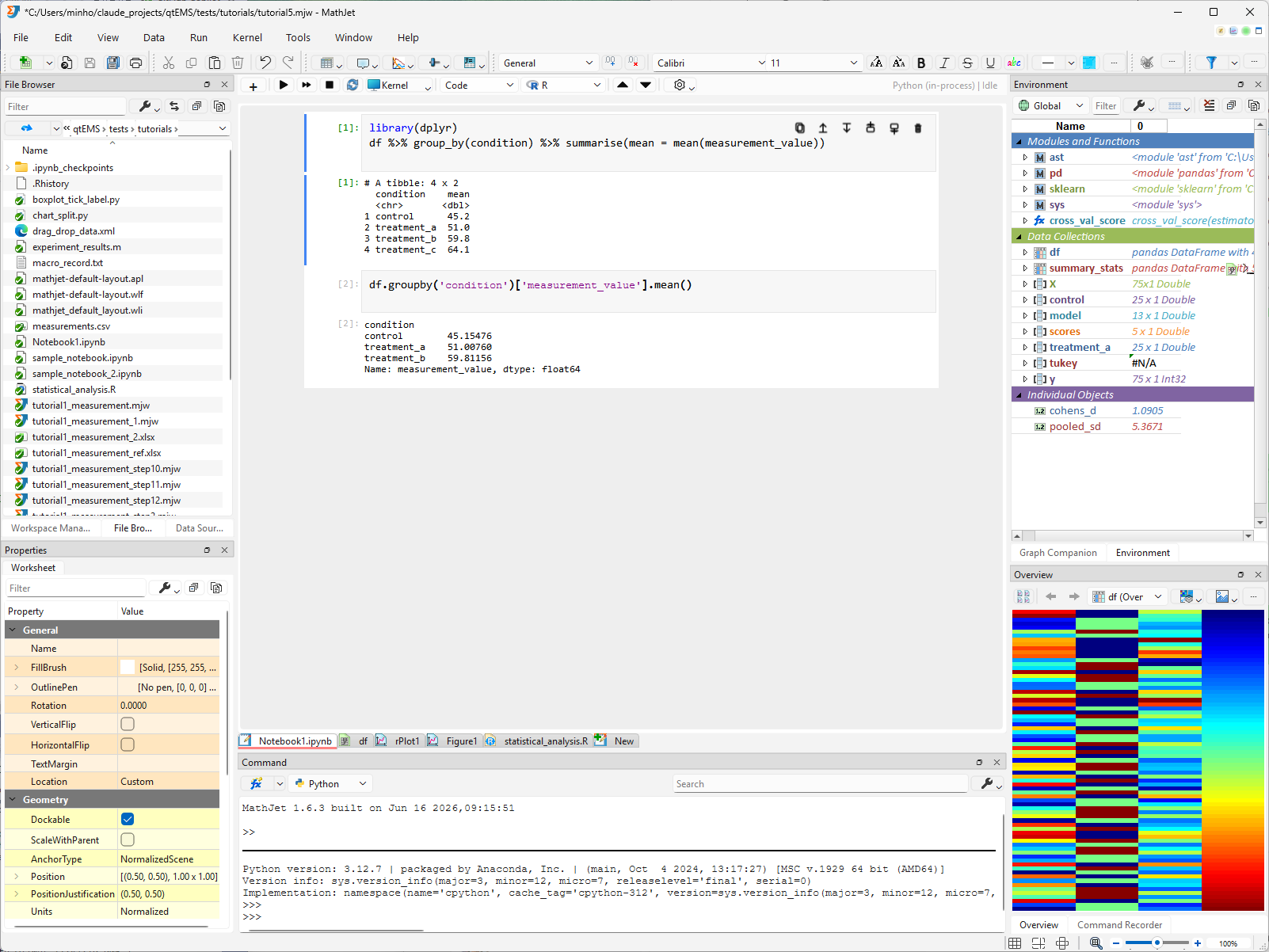
Step 9: R in a polyglot notebook

MathJet’s polyglot notebooks let you mix R and Python cells in a single .ipynb. This is useful when you want the notebook’s cell-by-cell structure but need both languages.

Create a new notebook: File → New → Notebook. The first cell defaults to Jet. Switch its language selector to R and type:

library(dplyr)
df %>% group_by(condition) %>% summarise(mean = mean(measurement_value))

Run the cell. R sees df from the script you ran earlier — it’s still in the shared data frame. The summary table prints below the cell.

Add another cell — it defaults to R (the current language). Switch its language selector to Python and type:

df.groupby('condition')['measurement_value'].mean()

Run it. Python produces the same group means from the same df. Two languages, interleaved cells, one shared namespace.

If you’ve moved a dplyr workflow to pandas (or vice versa), you know the conceptual mapping isn’t always obvious. Here both languages are describing the same operation on the same data — and you can pick whichever syntax fits your fingers, cell by cell.

You can add cells in Jet (MathJet’s MATLAB-syntax-compatible language) the same way. The language selector in each cell’s toolbar determines which interpreter runs that cell; the variables are shared across all of them.

Step 10: Save your work

Use File → Save to save the workspace as r-analysis.mjw. The workspace captures:

• The R script (embedded as a cached copy inside the .mjw)
• The interpreter state — every variable in R, Python, and Jet
• Any notebooks, worksheets, and charts you created
• Variable Editor state, Environment Pane expansion, and chart display settings

Close and reopen the workspace. The script, the variables, the charts, and the notebook all restore. The R interpreter reconnects and variables are available immediately — no need to re-run the script.

What you’ve learned

• How to open and run an existing .R file in MathJet’s embedded R interpreter, and that ggplot2 plots need to be run as a selection rather than sourced with the full script.
• That the output matches RStudio’s: same ANOVA p-values, same Tukey HSD intervals, same Cohen’s d — to within floating-point precision.
• That ggplot2 plots are intercepted and rendered as native interactive MathJet charts — zoomable, with the Graph Companion table showing boxplot statistics.
• How to inspect R workspace variables in the Environment Pane, with the Overview Pane picking shape-appropriate visualizations (scalar, line plot, heatmap, histogram) for whatever you click.
• How to open a data.frame in the Variable Editor and use it as a full spreadsheet alongside Excel formulas, with live round-trip linking to the R interpreter.
• That the Variable Editor’s column filters can apply to original data, removing rows from the interpreter’s data.frame — and that Ctrl+Z undoes the change.
• How to extend an R workflow with Python using the shared data frame — no rpy2, no reticulate, no serialization. R’s data.frames and Python’s DataFrames are the same objects in memory.
• How to mix R and Python cells in a polyglot notebook, with both languages sharing the same variable namespace.
• That MathJet’s .mjw workspace saves script state, interpreter variables, charts, and notebooks together — and restores them without re-execution.

Next steps

To see how the same shared-runtime model works for users coming from Jupyter, see Tutorial 4: Upgrading a Jupyter notebook with MathJet’s kernel.

To see it from the MATLAB side, see Tutorial 3: Bringing your MATLAB scripts into MathJet.

For a deeper look at the interactive chart features you saw on the upgraded ggplot2 plot, see Tutorial 6: Interactive plots — axis folding and data grouping.

To understand how variables flow between languages in more detail — the shared data frame, the py::/r::/jet:: qualifiers, mixed-language scripts — see Tutorial 2: Mixing languages in formula bar and scripts.

Troubleshooting

The script errors at library(dplyr) with “there is no package called ‘dplyr’”. MathJet uses your system’s R installation, so packages must be installed separately. Open a standard R console (or the Command Editor in R mode) and run install.packages("dplyr"). The same applies to ggplot2 and any other packages the script uses.

The ggplot2 boxplot doesn’t appear after running the full script. This is standard ggplot2 behavior — ggplot calls inside a sourced script build the plot object but don’t render it (same in RStudio). Select the ggplot(...) call and run it explicitly with Run → Run Selection (see Step 2).

The ggplot2 plot looks different from RStudio’s — different default colors, font sizes. That’s expected. MathJet renders ggplot2 output through its own plotting engine, which uses MathJet’s default chart styles rather than ggplot2’s. The data being plotted is identical; the visual styling differs. If you need RStudio-identical styling, MathJet preserves the theme and color settings you specify in the ggplot2 code (e.g., scale_fill_manual(values = ...), theme(text = element_text(size = ...))).

The ANOVA p-value or Tukey HSD intervals differ slightly from RStudio’s. Small differences at the last few decimal places are normal floating-point noise and depend on the linear-algebra backend. If the difference is substantive (different significance conclusions), that’s a real issue worth reporting — see Support.

Variables from R don’t appear in Python. Variable transfer through the shared data frame happens after each execution. If you’ve just run the R script and Python can’t see a variable, try running any R expression in the Command Editor first to trigger a sync. Not every R type transfers — data.frames, vectors, matrices, scalars, and lists all work; S4 objects, environments, and formulas may not. Check the Environment Pane for what made the trip.

install.packages() fails with a compilation error. Packages that require C/C++/Fortran compilation need a working toolchain on your system (Rtools on Windows, Xcode command-line tools on macOS, r-base-dev on Linux). Pre-compiled binary packages (the default on Windows and macOS from CRAN) install without a compiler.