Mixing languages in MathJet® — from formula bar to mixed-language scripts

30 minutes · Continues from Tutorial 1.

In Tutorial 1 you saw that cells, charts, and formulas all update live when any one of them changes. This tutorial shows the next layer: languages are fused too. You’ll use Excel, Jet (MathJet’s own MATLAB-syntax-compatible language), Python, and R in the same workspace — typed into cell formulas, run as Command Editor commands, and combined in a single mixed-language script file. Variables flow between languages automatically, through a shared data frame MathJet maintains in process memory.

Most environments make you pick a language up front. MathJet lets you change your mind per cell, per command, per segment — and the data doesn’t care which one.

Before you start

1. MathJet installed. Download if you haven’t.
2. Tutorial 1 completed. This tutorial picks up from first-analysis.mjw — the workspace you saved at the end of Tutorial 1. If you skipped that tutorial, go back and do it first; it takes 30 minutes and produces the data and chart this tutorial builds on.
3. Familiarity with reading short snippets in at least one of Python, R, or MATLAB-syntax. You don’t need to write any of them from scratch — the tutorial provides every line you’ll type. Recognizing patterns like numpy.mean(...), stats::quantile(...), or mean(x) is enough.

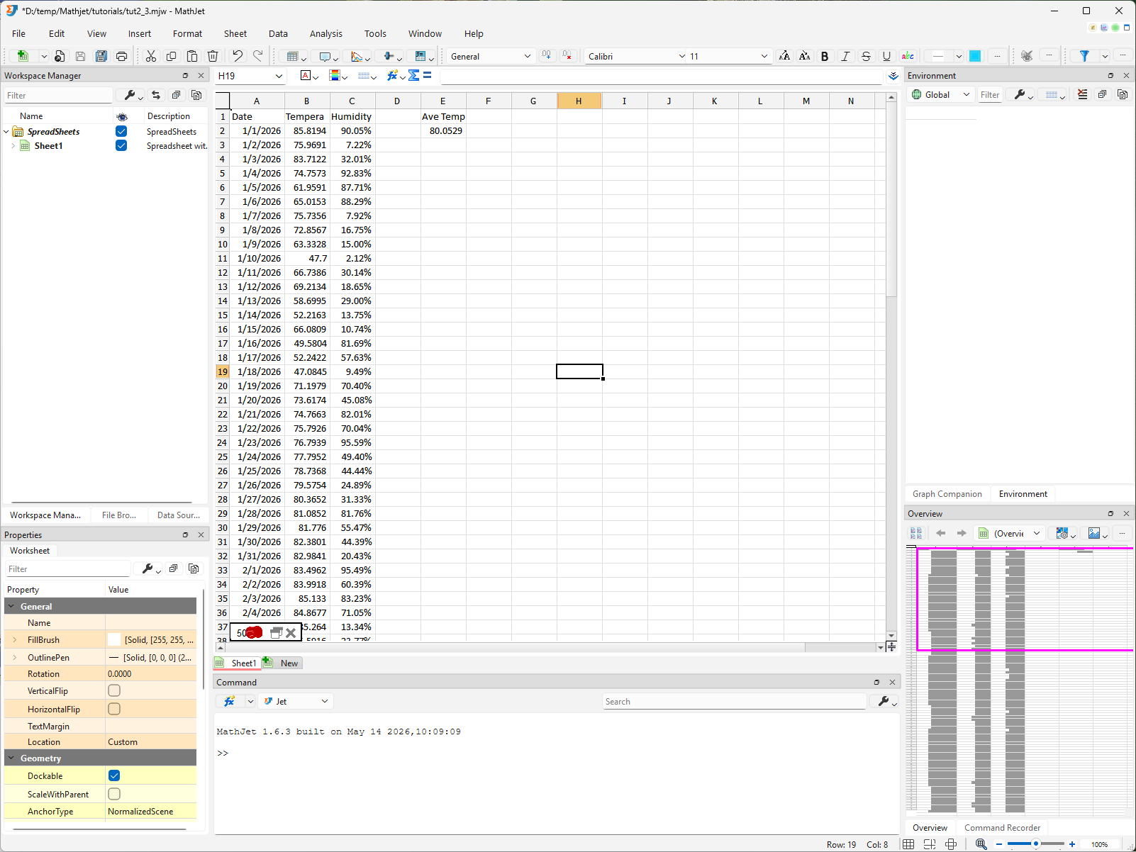
Step 1: Open the workspace from Tutorial 1

Open first-analysis.mjw. You should see:

• Columns A, B, C with 100 rows of date / temperature / humidity data
• Column D empty (the separator)
• Cell E2 holding =AVERAGE(B2:B101) with the label “Ave Temp” in E1
• The XY line chart floating inside the worksheet

A note before you start: The exact temperature and humidity numbers in columns B and C will differ from any screenshots below — they’re random draws from the distributions you set up in Tutorial 1, and your sample is different from anyone else’s. Any visual edits you made to the chart in Tutorial 1 (line width, color, splitting, etc.) will also carry over, so the chart may look different too. Everything in this tutorial works the same regardless; the cell locations and the operations are what matter, not the specific values.

Minimize the chart for a clean cell view. The next several steps live in the cell area, and you’ll want it unobstructed. Click on the chart to give it focus — the four semi-transparent buttons (Pin, Minimize, Maximize, Close) appear in its top-right corner. Click Minimize. The chart collapses to a small handle you can restore later by clicking it.

Bring the Environment Pane forward. The Environment Pane lives in the upper-right corner of the workspace, tabbed together with the Graph Companion you used in Tutorial 1. After reopening the workspace the Graph Companion is likely on top, so click the Environment tab to bring its pane forward. The Environment Pane is the GUI’s window onto the interpreter state — every user-defined variable that lives in Python’s, R’s, or Jet’s stack will appear here as a row. It’s empty right now, but it won’t stay empty for long; you’ll be watching it through the rest of the tutorial.

Step 2: The Command Editor and the embedded interpreters

Look at the Command Editor docked at the bottom of the workspace. At the top of the pane is a small drop-down — the language selector. By default it’s set to Jet, MathJet’s own MATLAB-syntax-compatible language. The dropdown also lists Python and R.

Each of these is a full interpreter running embedded in MathJet’s process. Switching the selector changes which interpreter the Command Editor talks to.

Try it. Make sure Jet is selected. Type 2 + 2 in the Command Editor and press Enter. The result 4 appears, computed by Jet.

Now switch the dropdown to Python. Type 2 + 2 and press Enter — the result is 4 again, but this time computed by Python. Switch to R, type 2 + 2, press Enter — 4, computed by R.

The math is the same. The point is that the language switch is instant, the dropdown is the only ceremony, and the interpreters are real — not stripped-down expression evaluators. You can import numpy, library(dplyr), define functions, hold state — anything you can do in a standalone interpreter.

Variables cross language boundaries automatically. With Python active, type:

x = numpy.array([10, 20, 30, 40, 50])

Switch to R. In the Command Editor, type x and press Enter — R shows the same array, now as an R numeric vector. Switch to Jet, type x — Jet shows the same array, now as a Jet matrix.

How? When the Command Editor changes language, MathJet captures the user-defined variables from the previous interpreter into its own data frame and loads them into the new interpreter’s stack on the way in. The variable name (x) stays; the value stays; the in-language type adapts.

Look at the Environment Pane. With x now in scope, the Environment Pane (upper-right) shows a row labeled x with a brief header describing its size and type. Click the small expansion handle next to the name — a two-column table opens directly below the header: the first column shows the indices ([0]–[4] if Python is the active language, [1]–[5] if R — each language uses its own indexing convention), and the second column shows the five values 10, 20, 30, 40, 50. At the same instant, the Overview Pane (lower-right) renders a small line plot of those five values — ready for the same exploration and editing you saw with cell-range nodes in Tutorial 1’s Workspace Manager. The Environment Pane and the Overview Pane react to every user-defined variable, regardless of which interpreter created it.

This shared data frame is the foundation for everything else in the tutorial.

Step 3: The polyglot formula bar

Cell formulas use the same model. You already have an Excel formula in E2 from Tutorial 1 — =AVERAGE(B2:B101) — recognized by its known uppercase function name and dispatched to MathJet’s Excel formula engine. Let’s add three more cells right next to it, each computing the same kind of value in a different language:

• Jet: click F2 and type =mean(B2:B101). mean isn’t an Excel function (Excel uses AVERAGE), so MathJet falls through to Jet — which has a mean function. Same value as E2.
• Python (auto-resolved): click G2 and type =numpy.mean(B2:B101). The parser sees numpy. and recognizes it as a Python module prefix, so it dispatches to Python. Same value again.
• R (auto-resolved): click H2 and type =base::mean(B2:B101). The base:: is R’s package-qualifier syntax — base is R’s core package, and base::mean is exactly R’s standard mean function, just namespaced explicitly. The parser sees package::function and dispatches to R. Same arithmetic mean as Excel’s AVERAGE, Jet’s mean, and Python’s numpy.mean.

Four cells, four languages, one column of source data, four computed values that all agree to floating-point precision. Three different embedded interpreters running in MathJet’s same process — Python, R, and Jet — arrive at the exact same number from the exact same array sitting in MathJet’s shared data frame. None of the cells care which language did the work.

When you need an explicit qualifier

The auto-resolution rules:

1. Excel formula functions (uppercase, on MathJet’s recognized list) dispatch to the Excel formula engine.
2. Anything else falls through to Jet — unless the expression starts with a recognized Python module name (e.g., numpy., pandas., scipy.) or uses R’s package-qualifier syntax (e.g., stats::), in which case it dispatches to Python or R respectively.

That covers most everyday cases. But some function names exist in multiple languages — mean, sum, log, length. When you type =mean(B2:B101), the parser routes to Jet because Jet has mean. If you specifically want R’s mean (which handles NA differently), you need an explicit qualifier.

That’s what the py:: / r:: / jet:: qualifier prefix is for. Drop down to row 4 and try three more cells:

• =py::numpy.std(B2:B101) in E4 — explicit Python qualifier. Same as =numpy.std(...) here because numpy. is already an unambiguous Python prefix, but the qualifier makes the dispatch obvious.
• =r::mean(B2:B101) in F4 — explicit R qualifier. Now the unqualified-mean ambiguity is resolved to R.
• =jet::log(B2) in G4 — explicit Jet qualifier. Useful when the expression starts with a name that could mean different things in different languages.

The rule of thumb: if your expression has a language-specific prefix (numpy., pandas., stats::, etc.), the parser will figure it out. If it doesn’t — if you’re calling a bare function whose name is ambiguous — add a qualifier.

Why the :: separator? R already uses :: for its package qualifier (stats::quantile), C++ and Rust use it for namespace resolution, and Julia uses it for module member access. It’s the most recognized “namespace operator” character pair in technical computing, and it doesn’t conflict with anything else in MathJet’s cell formula syntax. The py::numpy.mean(...) form composes cleanly when the inner expression itself uses :: (as in r::stats::quantile(...)).

Step 4: The worksheet as a REPL — variable cell blocks

This is where MathJet’s spreadsheet-and-scripting fusion gets distinctive. Type an assignment statement in any cell, and MathJet creates a variable on the active interpreter’s stack and renders that variable as an editable cell block right in the worksheet.

Set the Command Editor’s language selector to Python. Click cell G10 (somewhere with space below it). Type:

m = numpy.random.rand(5, 5)

Press Enter. A cell block appears in the worksheet, occupying G10:K15. The top row, G10:K10, is a header that shows the variable name m along with a brief description of its size and type (e.g., m — 5×5 double matrix). The five rows below it, G11:K15, display the 25 random values. The block has a thin frame and a small handle in its corner.

The cell block is a visual representation — not actual cell data. This is important and worth pausing on. No values were written into G11, G12, …, K15 in the spreadsheet sense. The variable m lives in Python’s stack (technically in MathJet’s shared data frame), and the block is just MathJet’s way of displaying that variable inline with the worksheet. Those cells aren’t real cells the way A2 or B5 are: you cannot reference G11 from a formula and expect to read m[0, 0], and the worksheet’s coordinate system has no addressable value at G11. The only way to refer to a value inside m is through the active language’s indexing syntax — m[0, 0] in Python, m[1, 1] in R, m(1, 1) in Jet.

To confirm: switch the Command Editor to Python and type m. The same array prints, with values matching the displayed block. Type m.mean() — gets the mean of the variable.

The block is editable — and editing it changes the variable. Click G11 (the top-left data cell — this is m[0, 0]), type a new value, press Enter. The Python variable m updates immediately; type m again in the Command Editor and the new value is there. You’re not writing to a cell; you’re using the block as a GUI surface for editing the variable. Edits to the header row are ignored — the header is metadata, not data.

The block is collapsible — and movable. Click the small handle in the block’s corner: the block collapses to a single cell showing just the variable name m. Click again to expand. While collapsed, you can drag the block’s border to relocate it anywhere on the worksheet — column N, row 50, wherever there’s space. The variable doesn’t move; only its on-screen placement does. A variable cell block has no fixed cell coordinates; it’s a floating view, not a region of the spreadsheet.

m also appears in the Environment Pane. Look at the upper-right: a new row m is in the Environment Pane alongside the x from Step 2. Expand it and you’ll see the same 5×5 table of values that’s rendered in the worksheet block — two views of the same variable. At the same time, the Overview Pane (lower-right) updates with a heatmap of m: a 5×5 grid of colored squares where each square’s color encodes its value, the same kind of visualization matplotlib’s imshow would produce for a 2D array. As m changes — whether you edit the worksheet block, the Environment Pane table, or the variable directly from the Command Editor — the heatmap repaints.

You can use the variable anywhere. Switch to R, type summary(m) in a new cell — R sees the same matrix (transferred to R through MathJet’s shared data frame) and prints summary stats inline. Switch to Jet, type size(m) in a cell — [5, 5].

A worksheet in MathJet is therefore two things at once: a spreadsheet and a REPL. Anything you can compute in a Command Editor command, you can type into a cell — and the variable shows up inline.

Step 5: Convert a cell range to a variable

The opposite direction is also supported: take data that’s already in cells, turn it into a programming variable, and operate on it with scripting commands.

Select the temperature column (cells B2:B101). Click Data → Create Variable from Cells (or its toolbar button). A dialog opens.

The dialog has these fields:

• Workspace — which workspace the variable will live in. Defaults to Global — the top-level scope of the current MathJet session, visible to every interpreter. Keep Global.
• Variable Name — the new variable’s name. Defaults to a short auto-generated name (e.g., a). Change it to temps.
• Data Type — the in-language type. Defaults to Automatic, which lets MathJet pick an appropriate type based on the cell contents and the active interpreter. For a column of numbers with Python active, Automatic produces a NumPy ndarray. Keep Automatic.
• Data Source — the cell range the variable reads from, written in Excel-style external-reference syntax: [workbook-name.mjw]SheetName!range. The field is pre-filled from your current selection, so it already reads something like [first-analysis.mjw]Sheet1!B2:B101. Leave it as is.
• Dynamically link variable to the data source — when checked (the default), the variable is a live link to the cell range: any edit in either the variable or the cells propagates to the other instantly. When unchecked, the variable is a one-time snapshot taken at creation. Keep it checked.
• Show variable in a new Variable Editor — when checked, opens a dedicated Variable Editor window for the new variable in addition to creating it. Leave unchecked for now.

Click OK.

The variable appears in the Environment Pane on the right. Confirm the link works:

• In the Command Editor (Python active), type temps.mean() — returns the same value as E2 (the =AVERAGE cell).
• Type temps[0] = 100. Press Enter. Look at the worksheet: B2 (the first temperature) is now 100. The chart’s temperature line shows a spike. E2 (the AVERAGE) recomputes.
• Edit B2 in the worksheet back to its original value. Type temps[0] in the Command Editor — the variable shows the new value.

A Python variable is a live view on a worksheet range. Edits flow either direction — change the variable, the cell updates; change the cell, the variable follows.

Step 6: A mixed-language script

This is the headline feature. A single script file can mix segments in Jet, Python, and R. MathJet runs each segment in its respective embedded interpreter and automatically transfers variables between segments through its shared data frame.

The segment boundary is marked with a # %% comment header (Jupyter-cell-magic style) followed by the language name.

Open a new script file: File → New → Script. Save it as analysis.jt in the same folder as the workspace. The script below uses Jet’s # operator to read from and write to worksheet cells — #B2:B101 reads the cell range B2:B101, and #L1 = "Mean" writes the text “Mean” to cell L1. (The # operator and its companion wrappers _f() and _t() are covered in full in the how-to guide Referencing and writing to worksheet cells from Jet commands.)

Type or paste the following:

# %% jet
% Pull the temperature data from the worksheet into a Jet variable.
% (The `#` operator reads from the active worksheet; this is the bridge
% from cells into the rest of the script.)
temps = #B2:B101;

# %% python
# `temps` was created in the previous segment (Jet) and transferred
# into Python's namespace. It's now a NumPy array.
import numpy as np
mean_temp = np.mean(temps)
std_temp  = np.std(temps)

# %% r
# `temps` is now an R numeric vector (transferred from Python's
# NumPy array through MathJet's shared data frame). `mean_temp` and
# `std_temp` came along too.
quartiles <- quantile(temps, c(0.25, 0.5, 0.75))

# %% jet
% All four variables (`temps`, `mean_temp`, `std_temp`, `quartiles`)
% are now in Jet's stack. Write a summary back to the worksheet.
#L1 = "Mean";    #M1 = mean_temp;
#L2 = "Std";     #M2 = std_temp;
#L3 = "Q1";      #M3 = quartiles(1);
#L4 = "Median";  #M4 = quartiles(2);
#L5 = "Q3";      #M5 = quartiles(3);

Save the file. Click Run (or press F5). The script editor highlights each segment in turn as it runs:

1. Jet segment reads the temperature column into a variable temps.
2. Python segment computes mean_temp and std_temp from temps.
3. R segment computes the three quartiles from temps and stores them in quartiles.
4. Jet segment writes labels and values to L1:M5 in the worksheet.

When the run completes, look at the worksheet: cells L1 through M5 now show the summary statistics. The mean was computed in Python. The standard deviation was computed in Python. The quartiles were computed in R. They all live in the same worksheet and reference the same source data.

Variable flow. At the end of each segment, MathJet captures every user-defined variable into its shared data frame. At the start of the next segment, the variables are loaded onto the new interpreter’s stack with names preserved and types adapted (Python ndarray → R numeric → Jet matrix, and so on). You don’t write any glue code; the dispatcher handles it.

Single-language scripts work too. A .jt file with no # %% headers runs entirely in Jet. Add a # %% python header at the top and it runs in Python. The header is opt-in.

Step 7: Save and reopen

Use File → Save to save the workspace. Close it. Reopen.

Everything restores:

• The data in columns A, B, C
• The formulas in row 2 (E2 through H2, from Step 3’s auto-resolved formulas) and row 4 (E4:G4, from Step 3’s qualifier examples)
• The labels-and-values block at L1:M5 (from Step 6’s mixed-language script)
• The variable cell block for m (the 5×5 random matrix), restored at whatever on-screen location you last left it
• The variables in the Environment Pane (temps, m, mean_temp, std_temp, quartiles)
• The script file analysis.jt
• The chart with all its display state

The Python, R, and Jet interpreters’ states are also captured — the variables they hold survive the save/reopen cycle. The .mjw workspace is a snapshot of all of it, in one file.

Embedded documents and the workspace cache. The .mjw package also stores cached copies of every external document the workspace references — the analysis.jt script you just saved, but also any .ipynb notebook, .m file, .xlsx source, image, or other linked asset. For each document, MathJet records both the absolute path and the relative path (relative to the workspace file). When you reopen the workspace, MathJet looks for each document in the absolute path first, falls back to the relative path next, and finally uses the cached copy from inside the .mjw if neither path is found. The practical consequence: you can move the workspace folder to a different machine — or send the single .mjw file to a colleague — and the script and data files still open, served from the cache. If the original files exist again later, MathJet picks them back up automatically on the next open.

What you’ve learned

• That MathJet ships with three embedded interpreters — Jet, Python, and R — running in the same process, with a shared data frame that automatically transfers variables between them.
• How to switch the Command Editor’s active language with the language selector dropdown.
• How the polyglot formula bar dispatches cell formulas: Excel formulas resolve first (by their uppercase function names), then Jet, then Python or R when the expression starts with a recognized module/package prefix.
• How to use the py:: / r:: / jet:: qualifier to explicitly dispatch a cell formula to a specific language when auto-resolution would be ambiguous.
• How an assignment statement in a cell creates a variable cell block — the variable lives on the active interpreter’s stack, and the worksheet shows it as a live, editable, collapsible block.
• How to convert a cell range to a variable with options for data type and live-linking.
• That Jet’s # operator lets scripts read from and write to worksheet cells — a bridge between the scripting world and the spreadsheet world, covered in full in the cell-operators how-to guide.
• How a mixed-language script with # %% language cell markers runs each segment in its embedded interpreter, with automatic variable transfer at each boundary.
• That MathJet’s .mjw workspace persists not just data and formulas but also interpreter state (every language’s variables), variable cell blocks, and script files.

Next steps

If your day-to-day work centers on a specific language, the tutorials that follow go deeper on each:

• MATLAB users: Tutorial 3: Bringing your MATLAB scripts into MathJet — Jet’s MATLAB-syntax compatibility, running .m files, the polyglot extension story.
• Python / Jupyter users: Tutorial 4: Upgrading a Jupyter notebook with MathJet’s kernel — opens existing .ipynb files, swaps the kernel, gains live variable inspection and editable DataFrames.
• R users: Tutorial 5: R / RStudio — bringing your R workflows into MathJet — shared-memory R, ggplot2 capture as native MathJet charts.

Two MathJet features touched on briefly in this tutorial deserve their own deeper walkthroughs:

• Dynamic variables — using => instead of = creates a variable whose value stays live-linked to the right-hand expression, even across languages. Type b => py::numpy.mean(a) * 2 and b recomputes whenever a changes. A how-to guide is forthcoming.
• The GUI Command Recorder — records your point-and-click actions as Jet statements you can replay or use as templates. A how-to guide is forthcoming.

Troubleshooting

My formula doesn’t auto-resolve to the language I expected. Use an explicit qualifier: =py::expression, =r::expression, or =jet::expression. The auto-resolution rules are convenient but not exhaustive — bare function names that exist in multiple languages always need the qualifier.

The variable cell block I just created looks wrong (e.g., transposed, scaled, or in the wrong cells). Confirm the variable’s actual contents from the Environment Pane or by typing the variable name in the Command Editor. A cell block is a view; if the underlying variable is what you expect, the rendering should be too. If you accidentally entered the assignment statement in a cell with neighbors that conflict with the variable’s natural extent, MathJet will refuse to render and show an error — clear the conflict or pick a different cell.

A variable I created in Python doesn’t appear in R after I switch languages. Variable transfer between languages happens at switch time. If you’re in a Command Editor session and the variable disappeared, you may have hit an unsupported type — not every Python type translates to R. Numerical arrays, lists, dicts (mapped to R lists), and pandas DataFrames (mapped to R data.frames) all work. Custom classes and language-specific objects may not. Check the Environment Pane for what made the trip.

The mixed-language script fails at a segment boundary. Most commonly: the variable name expected by the next segment doesn’t match what the previous segment created. The transfer is by name, so a typo in either segment breaks the link. Run the script segment-by-segment by placing the cursor in each segment and using Run Cell (or its hotkey) to isolate which boundary failed.

The #A1 reference returns an error in Python. That’s expected — # is Jet syntax. Switch the Command Editor’s active language to Jet for cell-reference work, or do the cell-reference work inside a Jet segment of a mixed-language script.